Epoch 8: Makemore, Part 5

Intro

Hi, this is chefcinnamon, in the previous epoch we learnt how to make mlp of makemore. In this epoch we learn more about Activations, gradients and BatchNorm.

Content: MLP Part 4

Let’s make our MLP again

1. dictionary:
   

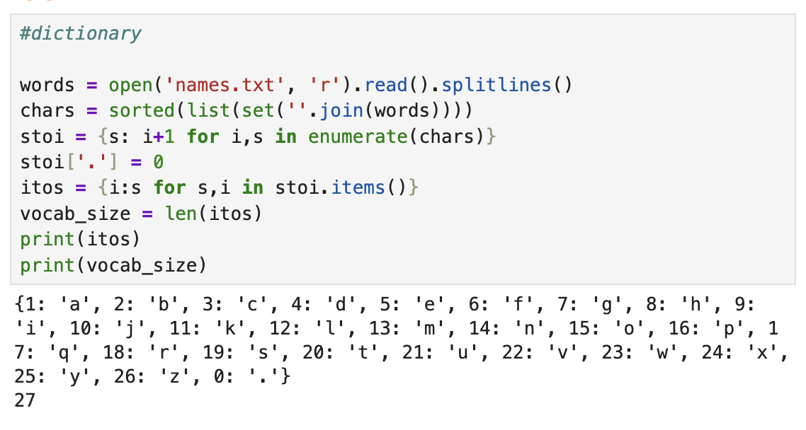
#dictionary 

words = open('names.txt', 'r').read().splitlines()
chars = sorted(list(set(''.join(words))))
stoi = {s: i+1 for i,s in enumerate(chars)}
stoi['.'] = 0
itos = {i:s for s,i in stoi.items()}
vocab_size = len(itos)
print(itos)
print(vocab_size)

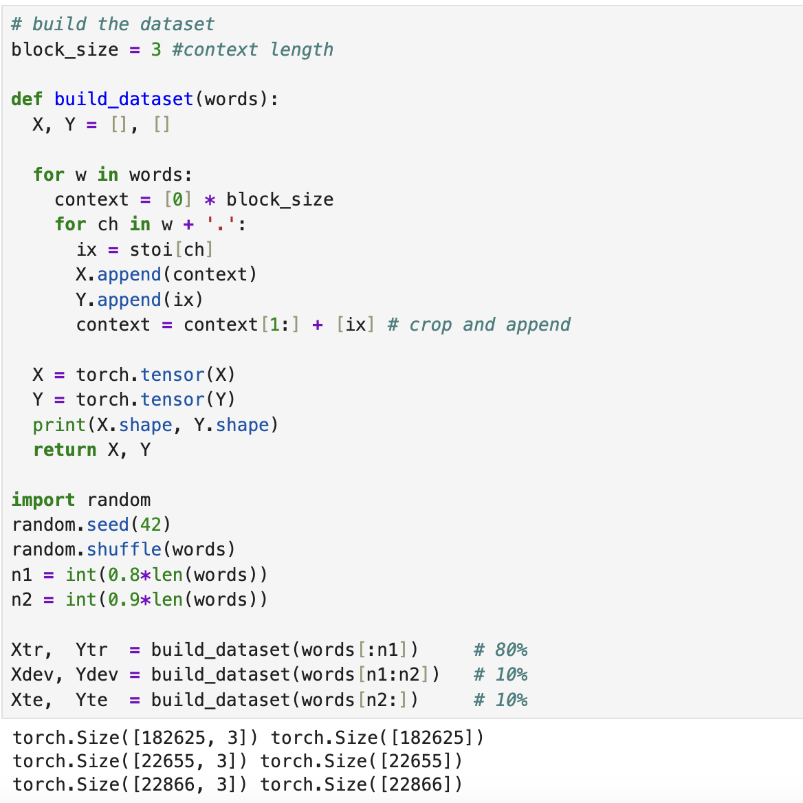
# build the dataset
block_size = 3 #context length

def build_dataset(words):  
  X, Y = [], []
  
  for w in words:
    context = [0] * block_size
    for ch in w + '.':
      ix = stoi[ch]
      X.append(context)
      Y.append(ix)
      context = context[1:] + [ix] # crop and append

  X = torch.tensor(X)
  Y = torch.tensor(Y)
  print(X.shape, Y.shape)
  return X, Y

import random
random.seed(42)
random.shuffle(words)
n1 = int(0.8*len(words))
n2 = int(0.9*len(words))

Xtr,  Ytr  = build_dataset(words[:n1])     # 80%
Xdev, Ydev = build_dataset(words[n1:n2])   # 10%
Xte,  Yte  = build_dataset(words[n2:])     # 10%

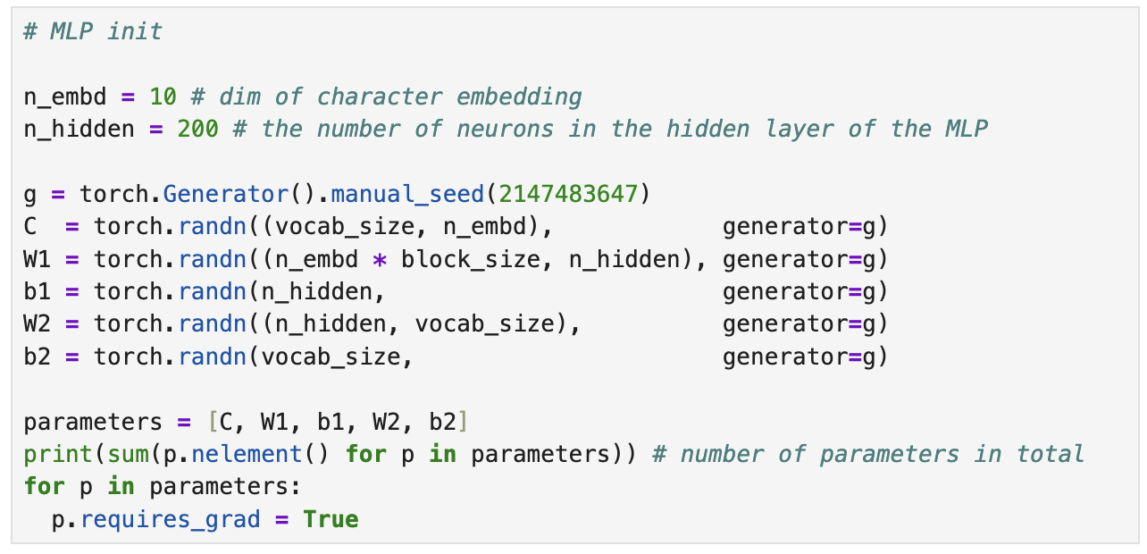
# MLP init

n_embd = 10 # dim of character embedding
n_hidden = 200 # the number of neurons in the hidden layer of the MLP

g = torch.Generator().manual_seed(2147483647)
C  = torch.randn((vocab_size, n_embd),            generator=g)
W1 = torch.randn((n_embd * block_size, n_hidden), generator=g)
b1 = torch.randn(n_hidden,                        generator=g)
W2 = torch.randn((n_hidden, vocab_size),          generator=g)
b2 = torch.randn(vocab_size,                      generator=g)

parameters = [C, W1, b1, W2, b2]
print(sum(p.nelement() for p in parameters)) # number of parameters in total
for p in parameters:
  p.requires_grad = True

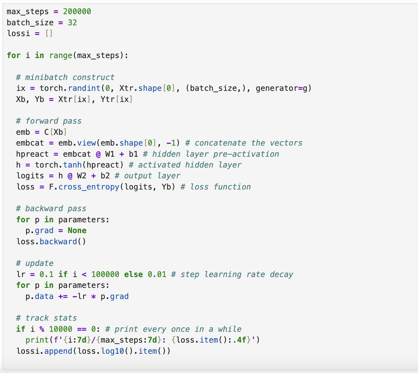
max_steps = 200000
batch_size = 32
lossi = []

for i in range(max_steps):
  
  # minibatch construct
  ix = torch.randint(0, Xtr.shape[0], (batch_size,), generator=g)
  Xb, Yb = Xtr[ix], Ytr[ix]
  
  # forward pass
  emb = C[Xb] 
  embcat = emb.view(emb.shape[0], -1) # concatenate the vectors
  hpreact = embcat @ W1 + b1 # hidden layer pre-activation
  h = torch.tanh(hpreact) # activated hidden layer
  logits = h @ W2 + b2 # output layer
  loss = F.cross_entropy(logits, Yb) # loss function
  
  # backward pass
  for p in parameters:
    p.grad = None
  loss.backward()
  
  # update
  lr = 0.1 if i < 100000 else 0.01 # step learning rate decay
  for p in parameters:
    p.data += -lr * p.grad

  # track stats
  if i % 10000 == 0: # print every once in a while
    print(f'{i:7d}/{max_steps:7d}: {loss.item():.4f}')
  lossi.append(loss.log10().item())
  

Note 1: (batch_size,) creates 1 dim(1,..)
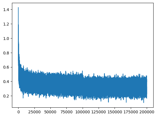
Note 2: for loss plotting we use log, due to better shaping for steps, more unified.

plt.plot(lossi)

Now lets compare loss in training and dev set

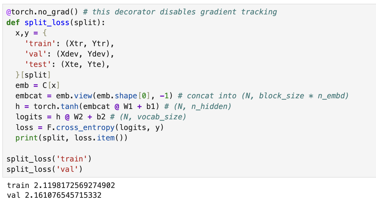
@torch.no_grad() # this decorator disables gradient tracking
def split_loss(split):
  x,y = {
    'train': (Xtr, Ytr),
    'val': (Xdev, Ydev),
    'test': (Xte, Yte),
  }[split]
  emb = C[x]
  embcat = emb.view(emb.shape[0], -1) # concat into (N, block_size * n_embd)
  h = torch.tanh(embcat @ W1 + b1) # (N, n_hidden)
  logits = h @ W2 + b2 # (N, vocab_size)
  loss = F.cross_entropy(logits, y)
  print(split, loss.item())

split_loss('train')
split_loss('val')

train 2.1198172569274902 val 2.161076545715332

We compare loss of training set and dev set to check if our model correctly is trained, and checks if or model works for the dev too.

If these 2 numbers are very different, it means something is wrong in the learning phase, we are either overfitting or underfitting.
Note: Dev set is not trained in the model at all.

Now let’s get sample names from our model:

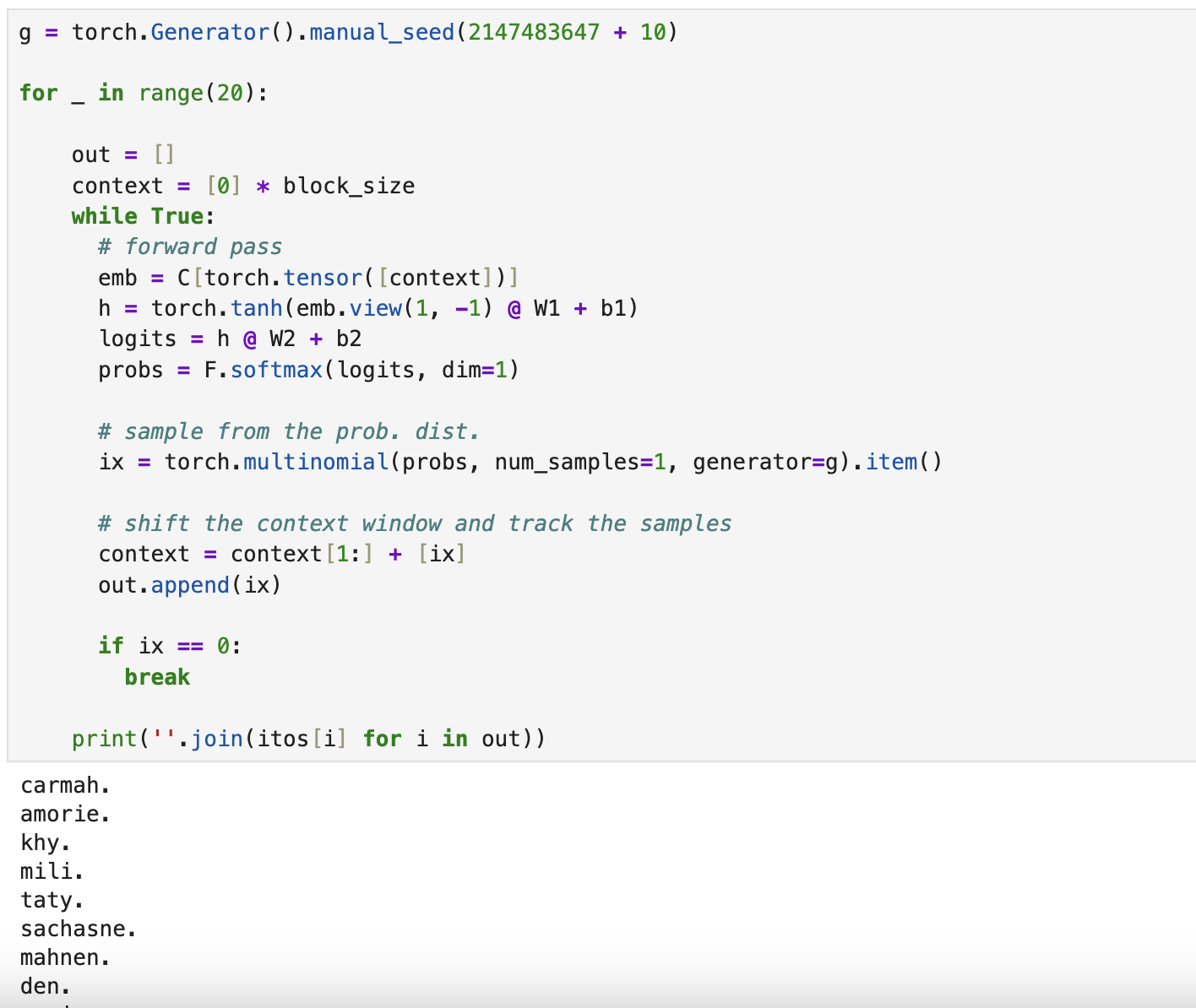
g = torch.Generator().manual_seed(2147483647 + 10)

for _ in range(20):
    
    out = []
    context = [0] * block_size
    while True:
      # forward pass
      emb = C[torch.tensor([context])]
      h = torch.tanh(emb.view(1, -1) @ W1 + b1)
      logits = h @ W2 + b2
      probs = F.softmax(logits, dim=1)
        
      # sample from the prob. dist.
      ix = torch.multinomial(probs, num_samples=1, generator=g).item()
        
      # shift the context window and track the samples
      context = context[1:] + [ix]
      out.append(ix)
      
      if ix == 0:
        break
    
    print(''.join(itos[i] for i in out))

Resources

An autoregressive character-level language model for making more things

GitHub: karpathy/makemore

The spelled-out intro to language modeling: building makemore

Google Colab Notebook

Google Colab: Makemore Part 5